The issues and concerns regarding the applicability of the 60/40 strategy are summarized in a recent front-page article in the Wall Street Journal penned by Akane Otani and Karen Langley titled: The Classic 60-40 Investment Strategy Falls Apart. ‘There’s No Place to Hide.’.
Although the list that follows is not meant to be exhaustive, here are some of the key arguments being made against the 60/40 allocation.
- It failed as a capital preservation strategy. It did not protect during the 2022 downdraft.
- It did not anticipate the 2022 debacle.
- The strategy only works when there is a negative correlation between the two asset classes
Capital preservation and downside protection
The case for the 60/40 portfolio focuses on the average return produced by the strategy. Its proponents argue that during market downdrafts the bonds help offset the losses generated by the stocks, the generalization being that the bond market will decline by less than the stock market. As far as downside protection is concerned, the biggest bang for the buck is delivered when the bonds and stocks are negatively corelated – something that investors will expect during periods of economic and market stress.
But how common are the negative correlation and/or stress periods? Figure 1 below shows stock and bond returns for the years 1987 through 2021. In all instances where stocks declined in value, bonds provided an offset. These results suggest that during market stress periods, the strategy capital preservation offered some downside protection.
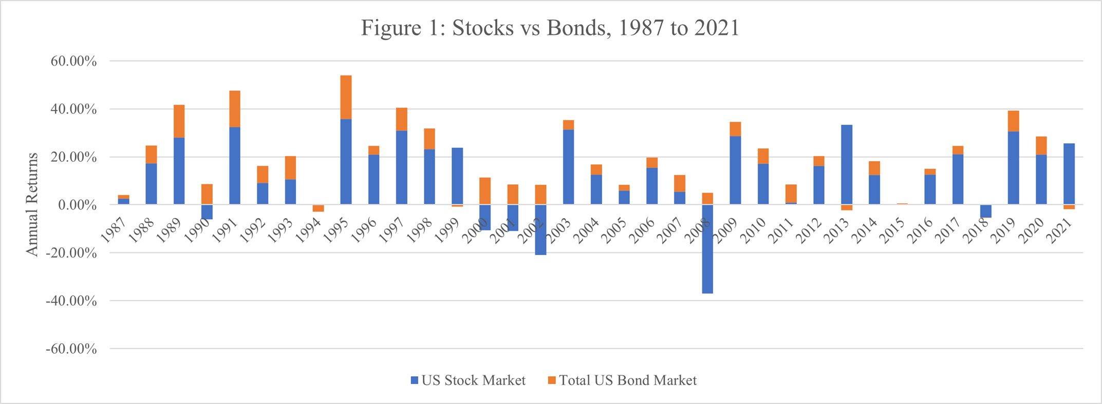
The negative correlation is a sufficient but not a necessary condition for bonds to improve the 60/40 portfolio returns relative to the pure stock portfolio returns. The necessary condition is that bond returns exceed stock returns, not move in the opposite direction of stock returns; this is a much lower bar to satisfy and happens with greater frequency. This is an important point worth repeating – relative performance is the necessary condition for capital preservation. Negative correlation is merely an extreme subset of the condition.
Given that there are two asset classes, there are four possible combinations of asset class performance:
- Bonds +, Stocks –
- Bonds +, Stocks +
- Bonds -, Stocks –
- Bonds -, Stocks +
Three of the possible return combinations above satisfy the condition of capital preservation:
- Stocks decline while bonds rise in value, a condition met during 1990, 2000,2001, 2002 and 2008. During those 5 years, the 60/40 portfolio outperformed stocks by 2210 points per year.
- Both bonds and stocks post positive returns, with the bond returns exceeding the stock returns. This condition was met during 2007, 2011 and 2015, and the 60/40 portfolio outperformed stocks by an average of 110 basis points.
- Both assets post negative returns with the stock decline exceeding the bond decline. During the 1987-2022 period only two years met this condition, 2018 and 2022, and the 60/40 portfolio outperformed the stock portfolio by an average of 160 basis points per year, see Table 1.
The data suggests that the negative correlation scenario (Scenario 1) generates the greatest bang for your buck by an order of magnitude of approximately 10x as compared to the other two scenarios studied. It is understandable, then, why negative correlation is often the key argument used in support of the strategy. However, the relative performance scenarios (Scenarios 2 and 3) still deliver excess returns, albeit more modest ones.
Therefore, in response to the first criticism posited by the article, “It failed as a capital preservation strategy. It did not protect during the 2022 downdraft”, our response is that while we can’t yet say how 2022 will turn out, thus far the year appears to be performing like Scenario 3. The first condition of capital preservation was satisfied, but the narrower condition of negative correlation was not.
This left us wondering, how effective is the 60/40 allocation as an insurance policy? The information reported in Table 1 shows that during 10 of the 36 years in the sample, or 27.78% of the time, bonds outperformed stocks. During those 10 years, the 60/40 portfolio outperformed the stock portfolio by an average of 11.7% per year.

Given that during the remaining periods stocks outperformed bonds, it follows that during the remaining years, or 72.22% of the time, stocks outperformed the 60/40 portfolio. Table 2 shows that during those 26 years the 60/40 portfolio underperformed stock portfolios by an average of 5.7% per year.

The question investors face is whether the excess returns of the bonds and the number of years the bonds outperform (in this case, 11.7% and 10 years respectively) generate returns large enough to compensate the investor for the 60/40 portfolio’s underperforming years (5.7% and 26 years). Our answer is no. The 60/40 portfolio’s frequency of underperformance is very high. If the answer was yes, then we would all be in 60/40 strategies. If it always outperformed, it would be the superior strategy. This result leads to the following question, under what conditions would an investor find the insurance offered by the 60/40 allocation beneficial?
In order to get a sense of the cost and benefits of the insurance afforded by the 60/40 portfolio we calculated the total excess returns generated by the 60/40 portfolio relative to the stock portfolio during the years that the bond returns exceed the stock returns, which equated to 10 years at 11.7% per year. These returns generate 117% worth of benefits over the 10 years. In contrast, the underperformance during the other periods is our proxy for the cost of the insurance. The 26 years at a 5.7% underperformance per year put the 60/40 portfolio cost of insurance at 148.2%. The calculation suggests that during the 1987-2022 period, the 60/40 allocation cost the portfolio 31.2% over 36 years or approximately 87 basis points per year.
However, as most investors know, cost is not the only factor in investment decision-making. Investment horizon matters as well.
Insurance and investor horizon
In order to get a sense of the possible downside of a worst-case scenario, we calculated the drawdowns for the 60/40 portfolio, the stock and bond markets during market stress periods, see Table 3.
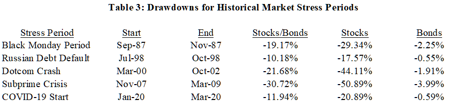
Stock market declines range from 17.57% to 50.89%. In contrast the corresponding decline for the 60/40 portfolio ranges from 10.18% to 30.72%. Hence the downdraft protection afforded by the 60/40 allocation ranges from 7.39% to 20.17% – a healthy degree of downside protection. But is that insurance worth it?
From an investor perspective, whether insuring a portfolio against stock market declines is worthwhile or not depends on a number of factors such as the magnitude of the downdraft, the recovery period and the investor horizon. Using the numbers in the previous section, it is apparent that an investor with a very long horizon, focused solely on the average return generated by his investments is better off self-insuring and choosing the 100% stock portfolio option instead of the 60/40 portfolio. Doing so improves his or her long run investment returns by 87 basis points per year.
But what about the investors with a shorter horizon? Can they afford to self-insure? Will they have enough time to recover from a market decline? If not, how much are they willing to pay in the form of reduced return for that insurance? In order to answer these questions, we calculated the drawdown and recovery periods for declines of more than 10% for the 60/40 portfolio and 100% stock portfolio, see Table 4. The Table identifies the beginning, end, and recovery period and the magnitude of the decline of the 100% stock portfolio and the 60/40 portfolio.
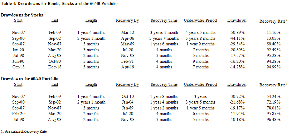
Since 2022 is the only bond market drawdown in excess of 10% and the year is not over, nor do we have an estimate of the recovery period, the bond market data is not reported, and we have excluded 2022 from the table above.
Comparing the 100% stock module to the 60/40 module, it is apparent that the episodes where stocks decline more than 10% includes the 60/40 episodes and then some. The declines of the 60/40 portfolio are less frequent and much smaller than the declines of the stock portfolio.
The data also show that for the episodes with recovery times in excess of 1 year, the recovery time for the 60/40 portfolio is much shorter than that of the stock market. These results imply that for each of the episodes, the recovery rate of return of the 60/40 portfolio exceeds that of the stock portfolio. These results lend support to the basic argument of downside protection used to justify the 60/40 allocation. This is particularly the case for investors with modest to short investment horizons. For investors with very long horizons the calculus is a bit different. If their horizon is long enough, they may be able to weather a large market decline if they are willing to wait. As already mentioned, for the 1987-2022 period, self-insurance resulted in an increase in the portfolio returns on the order of 87 basis points annually.
Thus, for the right investor with an adequate investment horizon, the 60/40 allocation offers the appropriate amount of insurance.
Black Swan?
The second point levied against the 60/40 allocation is that “It did not anticipate the 2022 debacle”. Did the strategy fail, or were the events of 2022 and the 60/40 portfolio performance simply beyond the realm of normal expectation? Said differently, was 2022 a Black Swan?
The ease of explanation of the advantage of a 60/40 strategy in terms of capital preservation and downside protection combined with its success during down stock market years fueled the popularity of the 60/40 strategy. Not surprisingly, it became one of the most basic and dependable ways of investing. Then 2022 happened.
The distribution of returns
As of the end of October, the US stocks and bonds are down 18.82% and 15.82% respectively. The 60/40 portfolio declined 17.62%. Although the 60/40 portfolio cushioned the decline as expected. The magnitude of the cushion was small in relation to the magnitude of the decline of the 60/40 portfolio.
The double-digit decline of the 60/40 portfolio throughout 2022 raised alarm bells among those who used it as a capital preservation strategy. Many devotees concluded that there was no place to hide; that the 60/40 portfolio had failed on the capital preservation front. Was the double-digit decline in returns a Black Swan event or is there a simpler explanation for the decline? In order to answer the question, we calculated the frequency of the different stock and bond return combinations and estimated the likelihood of these outcomes. Table 5 reports the frequency distribution of the four possible bond and stock return combinations.
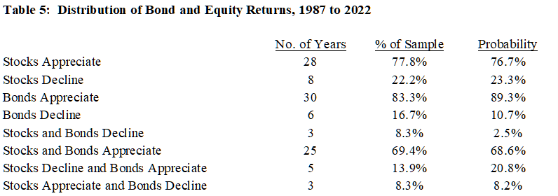
The data shows that stocks posted a decline 22.2% of the time, while the bonds posted negative returns 16.7% of the time. In turn, these frequencies ensured that the joint combination where one of the assets posted negative returns would be even less frequent. For example, only 3 times (or 8.3% of the time) did both stocks and bonds decline. Similarly, only 3 times did stocks appreciate while bonds declined. Only 5 times, or 13.9% of the times, did stocks decline and bonds appreciate.
The data in Table 5 show that the most frequent occurrence, at 69.2%, was one where both bonds and stocks posted positive stocks and bonds appreciate.
But is the frequency of the distribution of returns something unexpected given historical returns?
To answer the question, we performed a simple exercise. First, we calculated the stock and bond average annual returns and standard deviation. We then assumed that these returns were generated by two independent normal distributions. Next, we calculated the likelihood that each of the two asset classes would post a positive return during a year.
The probability for a positive stock return is estimated to be 76.7%, Column 3, Table 5, this is not too different from the 77.8% frequency posted by the real data. The likelihood of bonds posting a positive return was estimated at 89.3%, again, not too far off of the 83.3% posted by the real data.
The assumption that the two distributions are independent of each other allows us to compute the joint likelihood that both asset classes will post positive returns. This is nothing more than the product of the probability of each asset class posting a positive return. That number comes in at 68.5%, not too different from the realized 69.4%.
Our calculations put the estimated likelihood that each asset class independently posts a negative return at at 2.5%, a small probability but not insignificant, and not small enough to be considered a Black Swan. However, when focusing on the likelihood of the magnitude of the expected return of the 6-0/40 portfolio the answer may be different.
The CAPM framework: risk and expected returns
The estimated likelihood that stocks will post negative returns while the bonds post positive returns is estimated to be 20.8%, a large enough likelihood to prompt an investor to consider “buying” downdraft insurance. As documented here the 60/40 portfolio offers some downside/capital preservation protection. Whether that feature alone is enough to nudge an investor to the 60/40 portfolio depends on their investment horizon. The shorter the investor’s horizon the greater the likelihood that the investor will choose the 60/40 portfolio to deliver the desired protection. But focusing solely on the expected return misses a potential benefit of the 60/40. It ignores the risk reduction possibility of the 60/40 portfolio. The last few decades, developments in modern portfolio theory provide a framework for addressing the way risk can affect expected returns. We have the Capital Asset Pricing Model (CAPM) which looks at the relationship between an investment’s risk and its expected market return. These developments help us answer some of the questions that remain regarding the desirability of the 60/40 allocation in the context of the CAPM.
CAPM and the 60/40 allocation
The lay argument in favor of a 60/40 allocation implicitly assumes that the two assets are negatively correlated. But as the 1987-2022 data show, negative correlation, when the returns of one asset class is positive and the other negative, only occurs 22.2% of the time. Hence, if two assets are negatively correlated and move in opposite directions, as the justification for the 60/40 allocation suggests, the volatility of a portfolio consisting of these two assets would be much lower than that of a portfolio consisting of only one of the assets. The latter represents an example of a risk that can be diversified away by combining it with other assets in the portfolio. But what about the remaining 77.8% of the time?
A major insight of the CAPM is that not all risks should affect asset prices. The implication being that if the asset does not add to the volatility of the portfolio, it should not be priced for risk, or more plainly, investors would not demand additional return or a premium over and above the current expected return. But the CAPM shows that a negative correlation between two asset classes is not the only way to reduce the overall volatility of a portfolio. All that is required is that the assets not be perfectly correlated, i.e., that the correlation is different from 1. Hence, viewed from this perspective, negative correlation assumed by the simple 60/40 marketing strategy previously mentioned is a sufficient but not a necessary condition for the reduction of the volatility of a portfolio consisting of two non-perfectly correlated assets. Therefore, the CAPM offers a less restrictive way to build less risky portfolios than one that simply selects negatively correlated assets.
It offers a powerful and intuitive explanation about how to measure risk, and the relationship between expected returns and risk. It offers a clear risk return tradeoff mechanism and is an appropriate technique to optimize an investment strategy. According to the CAPM, the only risk that should be priced is the risk that cannot be diversified away, the residual risk or systematic risk. The CAPM is firm on this point. What should matter to the investor, therefore, is the incremental volatility on the overall portfolio volatility, not the individual investment volatility. When considering adding an asset to a portfolio, the asset may impact both the portfolio return as well as the overall volatility. Hence the investor has to determine whether the incremental investment adds to the risk or volatility as well as the return of the overall portfolio. In turn, the investor then has to decide whether the incremental return is sufficient to compensate the investor for any added risk to the overall portfolio.
Nobel Prize winner Bill Sharpe has come to the rescue of investors who must perform this task. Because of him, we now have the Sharpe Ratio at our disposal. This well-known formula is useful for evaluating potential investments and determining when to add additional assets to a portfolio. If a potential addition to a portfolio improves the Sharpe Ratio, the asset in question adds to the return of the portfolio over and above the return required to compensate for the increased volatility (i.e., risk) of the new portfolio. Adding the asset improves the overall portfolio performance.
The portfolio optimization process leads the investor or manager to search for an efficient portfolio, defined as a portfolio that contains returns that have been maximized in relation to the risk levels that individual investors desire. Once the efficient portfolios are identified, the investor searches for the portfolio with the highest Sharpe Ratio. In the aggregate, in a market that is in equilibrium, where the number of winners and losers must balance out, adding one additional asset class or stock does not increase the portfolio’s risk-return ratio. This means the portfolio containing risky assets with the highest Sharpe Ratio must be the market portfolio. It also turns out, on average, stocks account for about 60% of the overall market capitalization and fixed income accounts for about 40% of the liquid asset market valuation. All of this is a very roundabout way to show that the 60/40 allocation is an efficient allocation with a higher Sharpe Ratio than its component asset classes.
Using the CAPM prism to interpret the data
Although not explicitly discussed, the initial justification for the 60/40 implicitly assumes that the bond component reduced the portfolio volatility. The addition of the bond component also raises the possibility that the bond allocation may also reduce the portfolio average return, but the CAPM argues that as long as the Sharpe Ratio increases, the reduction in volatility more than compensates the investor for the reduction in returns.
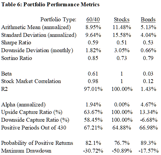
Table 6 reports a variety of statistics used to evaluate the performance of the 60/40 portfolio vis-à-vis a 100% stock portfolio and 100% bond portfolio. The data show that the average return and volatility of the 60/40 portfolio is bookended by the returns and volatility of the 100% equity and 100% fixed income portfolios, Rows 1 and 2, respectively, in Table 6. To determine whether the reduction in volatility is large enough to compensate the investor for the lower return we calculated the Sharpe Ratios of the three portfolios or asset classes. At 0.59, the Sharpe Ratio for the 60/40 is higher than the 0.51 posted by the equity portfolio, and the 0.53 posted by the fixed income portfolio. Therefore, it is safe to conclude that adding equity to a fixed income portfolio and vice versa is a worthwhile endeavor. On a risk adjusted basis, the addition of bonds to the portfolio improved portfolio performance. Notch one for the 60/40 portfolio.
Given the emphasis on downside protection and capital preservation, we need to focus on the portfolios’ downside deviation. The statistics are reported in Row 4 of Table 6. Again, the average downside deviation of the 60/40 portfolio is bookended by the downside deviations of the 100% stock and 100% bond portfolios. Once again, these results raise the question as to whether the reduction was worth it. To answer this, we calculate the Sortino Ratio, best described as a Sharp Ratio for the periods with negative returns. The data reported in Row 5 shows that the 60/40 portfolio has a higher Sortino Ratio than the other two portfolios, the conclusion being that adding bonds to the 60/40 portfolio provided incremental downside protection that more than compensated for any reduction in the portfolio’s average returns.
Ultimately, investors focused on retirement care about wealth accumulation. So, it is important to understand how the 60/40 allocation relates to the stock portfolio, i.e., its covariance with the stock markets. If in fact the bond portfolios are uncorrelated to the stock portfolios, their beta should be at or near zero, the stock market beta being 1. Given a zero beta for bonds and a beta of 1 for stocks, we expect the beta of the 60/40 portfolio to be 0.6. Table 6 shows our estimated 60/40 portfolio beta to be 0.61. In theory we also expect the bonds to be uncorrelated to stocks and thus expect the 60/40 portfolio to move with and mirror the stocks’ fluctuation with the magnitude of these fluctuations approaching 60% of the stock fluctuations. Hence, we look for the equities to have a near 100% correlation to the 60/40 portfolio. The data reported in Table 6 indicates that that is the case. The results are exactly what the CAPM suggests.
What accounts for the positive alpha?
An interesting result reported in Table 6 is that both the 60/40 and bond portfolios have positive alphas. That is, a return higher than the one expected under the CAPM.
Given the bond portfolio’s zero beta, we expect the 60/40 portfolio to capture 60% of the upside and downside of the stock portfolio. Any deviation from the 60% capture is attributable to the bond capture plus any bond-stock interaction. The 60/40 portfolio’s upside capture is estimated to be 63.67%. The upside capture in excess of 60% means that the bonds added to the returns. Similarly, a downside capture below 60% means that the bonds cushioned the stock decline and the portfolio would decline by less than 60% of the stock portfolio. These calculations explain the deviations of the upside capture from the theoretical 60%, and largely account for the excess return or estimated alpha. The positive periods batting average of the 60/40 is higher than that of the weighted average of the stock and bond portfolios. The higher batting average points to a positive interaction between the stocks and bonds, a result consistent with the upside and downside capture ratios as well as the Sharpe and Sortino Ratios.
Finally, we need to make a very important point. The estimated alpha are not a skill based excess return normally attributed to a positive alpha. Instead, the estimated risk adjusted excess returns are not the traditional alpha, they reflect a systematic source of returns that can be captured predictably at little or no cost.
Did the 60/40 strategy fall apart in 2022?
The traditional sales pitch for the 60/40 portfolio is that when stocks have a bad year bonds usually do better which helps offset those losses. The CAPM shows that while a negative correlation is the easiest way to reduce the volatility of a portfolio, it is not the only way. As long as the correlation between assets is not perfect, adding bonds to a stock portfolio could, in fact, reduce its volatility and reduce its potential drawdowns. The data reported in Table 3 supports this point of view. Stocks and bonds have posted negative returns during “market stress periods” — Black Monday, the Russian debt default, the dot-com crash, the subprime crisis and most recently the Covid-19 pandemic. Notice that during the market stress episodes, the 60/40 portfolio performed admirably even though both asset classes posted negative returns, i.e., there was a positive correlation between the two asset classes. Although a negative correlation ensures that the 60/40 strategy would dampen the stock market declines, the data reported in Table 3 shows that this is not a necessary condition for the 60/40 portfolio to deliver. The key to the bonds’ cushioning effect is the differential return between stocks and bonds. As long as the magnitude of the negative bond return is less than the magnitude of the stock returns, the 60/40 allocation will cushion the stock decline.
Some financial writers have argued that during 2022 the 60/40 portfolio fell apart, but we beg to differ. As of the end of October, the broad US stock market was down 18.82% while the broad bond market was down 15.82% and the 60/40 portfolio was down 17.62%. The 60/40 portfolio did cushion the market decline as the proponents of the strategy argue. The implicit complaint of many of the people who argue that the 60/40 portfolio has failed is that it only reduced the stock decline by 120 basis points. Essentially the complaint is that the differential return between the two asset classes was not larger. But the 60/40 portfolio is silent regarding the rate of return differential between stocks and bonds and thus the magnitude of their weighted average. Qualitatively, the 60/40 portfolio performed as expected. Viewed from this perspective it would be wrong to conclude that the strategy is broken.
Was 2022 a Black Swan event for the 60/40 portfolio?
In contrast to our earlier analysis that a decline of each of the asset classes was not a Black Swan event, our data points to 2022 being a Black Swan event for the 60/40 portfolio. Here is why. Assuming that the sample average annual returns and standard deviation for the 60/40 portfolio are the result of repeated drawing from a normal distribution, we estimate the likelihood of the 60/40 portfolio return decline to the level experience during 2022 to be 0.29% – a probability that falls well below the range of normal expectation. One way to put the 2022 outcome in perspective is to liken the decline to a 300-year flood – a flood that on average occurs once every 300 years. Additionally, what makes it a Black Swan is not the fact that the 60/40 portfolio delivered a negative return. What makes is such a unique and unexpected event is the magnitude of the decline.
Should investors abandon the 60/40 approach?
The data reported in Table 4 and 5 documents that during the major drawdowns of the last several decades the 60/40 portfolio has posted average declines in the neighborhood of 60% of the decline in stocks. Furthermore, for recoveries lasting more than 1 year, the recovery rate of the 60/40 portfolio has been approximately half of the recovery period of stocks. If, as we believe, the process is not broken, this is not the time to abandon the 60/40 portfolio. Stay the course and expect a faster recovery with the 60/40 portfolio.
Yes, 2022 has been a tough year, but as we have argued – the year was akin to a 300-year flood. We look forward to sunny skies and higher ground in the years ahead

IMPORTANT DISCLOSURES
The information in this report was prepared by Timber Point Capital Management, LLC. Opinions represent TPCM’s and IPI’s opinion as of the date of this report and are for general information purposes only and are not intended to predict or guarantee the future performance of any individual security, market sector or the markets generally. IPI does not undertake to advise you of any change in its opinions or the information contained in this report. The information contained herein constitutes general information and is not directed to, designed for, or individually tailored to, any particular investor or potential investor.
This report is not intended to be a client-specific suitability analysis or recommendation, an offer to participate in any investment, or a recommendation to buy, hold or sell securities. Do not use this report as the sole basis for investment decisions. Do not select an asset class or investment product based on performance alone. Consider all relevant information, including your existing portfolio, investment objectives, risk tolerance, liquidity needs and investment time horizon.
This communication is provided for informational purposes only and is not an offer, recommendation, or solicitation to buy or sell any security or other investment. This communication does not constitute, nor should it be regarded as, investment research or a research report, a securities or investment recommendation, nor does it provide information reasonably sufficient upon which to base an investment decision. Additional analysis of your or your client’s specific parameters would be required to make an investment decision. This communication is not based on the investment objectives, strategies, goals, financial circumstances, needs or risk tolerance of any client or portfolio and is not presented as suitable to any other particular client or portfolio. Securities and investment advice offered through Investment Planners, Inc. (Member FINRA/SIPC) and IPI Wealth Management, Inc., 226 W. Eldorado Street, Decatur, IL 62522. 217-425-6340.
Recent Comments