Friedman taught us that inflation is, and always has been, a monetary phenomenon. Too much money chasing too few goods. He also argued that M2 is the appropriate measure of the quantity of money circulating in the economy while real GDP denotes the quantity of goods. If inflation is too much money chasing too few goods, an M2 growth rate in excess of real GDP growth leads to an excess money supply. To restore monetary equilibrium, the price of money in terms of goods, or what is commonly defined as the purchasing power of money, has to change to eliminate any excess demand or supply of money.
The recent slow economic performance allows us to make a simplifying assumption of a flat real GDP. In simple terms this means no change in the economic demand for money. Doing so allows us to focus solely on the changes or shifts in the money supply conditions, i.e., M2 growth rate, as our proxy for the excess money supply. This in turn allows us to determine the inflation rate needed to restore equilibrium in the money market.
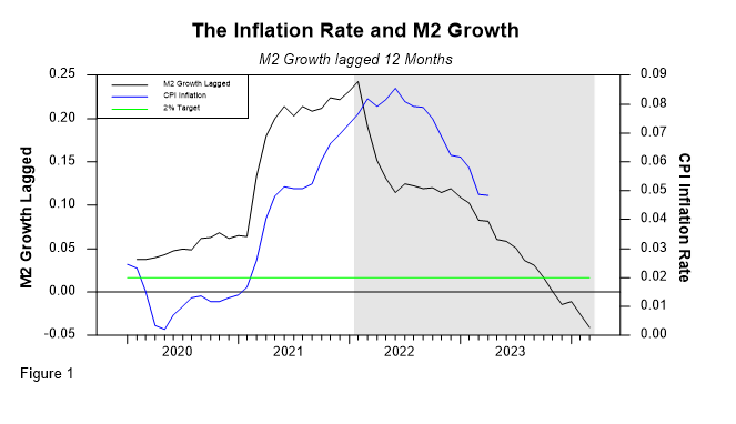
Figure 1 documents the relationship between the inflation rate and the M2 growth rate lagged one year. The data clearly supports the monetarist hypothesis. First the data supports the monetarist view of a lagged monetary response. Second, since M2 growth precedes the inflation rate, it seems reasonable to conclude that M2 growth causes the inflation rate. Third, given the assumption of no change in demand, i.e., a near flat real GDP growth, the M2 growth rate is our proxy for an excess money supply. Fourth, too much money leads to a higher inflation rate. Thus, we have an explanation for the surge in the inflation rate in the aftermath of COVID. The surge in M2 growth is evident to the naked eye. Fifth, the Fed appears to have admitted its mistake and its decision to reduce its Balance Sheet and Monetary Base appear to have reduced the growth rate of the broad monetary aggregate, M2, and consequently the inflation rate.
Going forward, the fact that M2 growth rate is negative, combined with the assumption of a lagged monetary response, means that the inflation rate is expected to continue its decline. In fact, the relationship reported in Figure 1 suggests that if the M2 growth rate continues on its current path there is a strong possibility that the US inflation rate will approach the Fed’s 2% target rate by the November 2024 election.
Who controls M2?
The analysis in the previous section implicitly assumes that the Fed controls or significantly impacts the quantity of M2. But is that the case? The textbook representation of monetary and banking systems assumes that the Federal Reserve Bank controls the monetary base. It does so by conducting open-market operations: When the Fed wants to increase the greenbacks circulating in the economy, it buys government securities in the open market and pays for them by printing money. Similarly, when the Fed wants to reduce the quantity of greenbacks circulating in the economy, it sells government securities to the public. In exchange it receives greenbacks which the Fed takes out of circulation. Hence the open market operation is the mechanism by which the Fed alters the greenbacks circulating in the economy, i.e., the monetary base. But that is only one component of the monetary aggregates. Under a fractional banking system, the greenbacks or monetary base have two uses. One being as Currency in Circulation and the other being as Reserves backing bank Deposits. Although under the current system, banks do not have any legal reserve requirements, prudence and other regulations induce the banks to voluntarily hold some reserves backing the deposits and loans of the banking system.
A simple numerical example illustrates the mechanics of the banking system, monetary and credit markets, and credit creation mechanisms.
Let’s assume a banking system that has a monetary base of $10 where people decide to hold $3 in cash, or currency in circulation, and the remaining $7 is used by banks as reserves backing deposits.
Next, we assume that the banks find it prudent to hold 20% in reserves for every $1 worth of deposits. Under these conditions every $1 worth of reserves can back up to $5 worth of deposits, the bank’s liabilities. This math is easy, that means the bank’s deposits are equal to $35 ($7 in reserves multiplied by $5). Given double-entry bookkeeping, assets must equal liabilities, the banks will also hold an equal amount of assets, $35 in this example. We started out with $7 worth of reserves and the difference between the deposits, $35, and the reserves denotes the loans made by the banks, i.e., $28.
To summarize, $7 worth of reserves back $35 worth of deposits and $28 worth of loans. Since M2 is defined as the amount of currency in circulation held by the private sector, $3, plus the demand deposits, $35, M2 adds up to $38 and the bank credit in this example is $28.
Double entry bookkeeping tells us that the bank’s assets and liabilities have to match. As we have shown, under a fractional reserve banking system, deposits and bank credit are intertwined. Similarly, the quantity of money, M2, circulating in the economy is related to the monetary base as well as the interaction between the deposit and credit creation by the commercial banks.
The Fed’s ability to control M2 rests on its ability to simultaneously control the monetary base and, through regulations, the banking system’s credit creation, i.e., the loan multiplier. An extreme and common assumption made by some textbooks and many analysists is that the loan or credit multiplier is constant. Under that assumption the quantity of money, M2, will be proportional to the monetary base, the proportionality factor being called the money multiplier. But is that the case? Figure 2 shows the relationship between the monetary base, the bank credit creation, i.e., loans and deposits, and M2.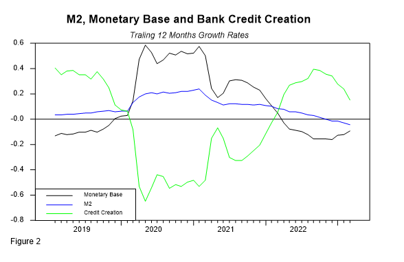
Figure 2 shows that when the monetary base appears to expand too fast, credit creation declines to offset some of the undesired increases. Similarly, when the monetary base growth rate declines credit creation increases. Although in theory it is possible that the banking system could completely offset the undesired increases in the monetary base, in practice credit creation changes are never large enough to completely offset changes in the monetary base. The net effect being that the M2 growth rate tracks the monetary base growth rate, although the magnitude is muted. The most one can say is that bank credit creation dampens the “undesired” changes in the monetary base. Hence even if the Fed controls the monetary base, its control of M2 is not absolute. The data suggests that the banking system has enough flexibility to offset and ameliorate some of the undesired changes in the monetary base affected by the Fed, at least partially. Thus, Fed monetary policy must take into consideration the variables that impact the banking system’s credit creation if it is to control M2.
Money and Credit equilibrium
The numerical example previously discussed documents how deposits and loan credit creation are linked together through the fractional reserve system. By altering the reserve deposit ratio, banks are able to alter their deposit and credit creation independent of the amount of reserves that they hold. The banks’ ability to alter the reserve deposit ratio allows the banks to offset undesired increases in the monetary base and to magnify the desired increases. In doing so the banks weaken the Fed control over M2.
The discussion also suggests that while the two markets — money and bank credit– are interconnected, they are different markets. This means that in order to determine the equilibrium conditions of each market, we need to track the demand for money and credit as well as the supply of money and credit. We must also keep their interconnection, due to the fractional reserve system, in mind during our analysis. Overall equilibrium yields market clearing conditions for each one of the markets.
- The equilibrium in the money market requires the quantity of money, M2, and the price of money or purchasing power of money, i.e., the inverse of the CPI.
- The bank credit equilibrium requires the quantity of bank credit, i.e., loans, as well as the market clearing price of the loans, the market clearing interest rate.
Interaction between the money and credit markets:
The fractional reserve banking system introduces a series of interconnections between the money and credit markets that cannot be ignored because they have a predictable impact on the overall equilibrium conditions. The different interactions provide a direct link between the two markets and as a result disturbances in one market will impact that market’s equilibrium conditions, filter through and impact the other market’s equilibrium too. Let us consider the impact of a flight to quality that results in an excess demand for currency in circulation.
The effects of the increase in currency holdings on M2 and the inflation rate: Holding the monetary base constant, the increase in currency holdings means a reduction in bank reserves. Thus, everything else the same, the reduced bank reserves result in a lower quantity of bank deposits and bank loans. Given the fractional reserve banking system we can then argue that a one dollar increases in currency holdings leads to a multiple reduction in demand deposits equivalent to the inverse of the reserves backing deposits. This means that the increase in currency holdings will be smaller than the decline in deposits. Since the quantity of money is the sum of the currency in circulation plus demand deposits the conclusion being that the flight to quality leads to a reduction in M2.That in turn results in an excess demand for money due to the shortage of money. The market clearing condition requires that the price of money increase. Since the price of money is the inverse of the CPI, that means a decline in the price level and therefore an increase in the purchasing power of money. In dynamic terms the excess demand for money due to the increase in demand for currency will have a delayed or lagged effect that results in a decline in the inflation rate.
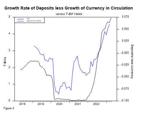
The effects of the increase in currency holdings on bank deposits and the short-term interest rate. The flight to quality alters the currency and deposit market equilibrium. Given our view that, all else the same, the choice between currency and demand deposits depends on the opportunity cost of holding cash, the shortage of deposits induce an increase in the opportunity cost of holding cash. That is the short-term interest rate increase leading to an increase in the deposit-to-currency ratio that partially undoes the initial reduction due to the flight to quality. That is, the interest rate paid on the deposits will be positively correlated to the change in the deposits to currency holdings in the economy. The data in Figure 1 documents the positive correlation between T-Bills and the growth rate of demand deposits less the growth rate in currency holdings. During a flight to quality, as occurred during the COVID episode, Figure 3 shows that the currency deposit ratio declined as did short-term interest rates.
The effects of the increase in currency holdings on bank loans or credit creation and the long-term (i.e., loan) interest rate. Given the monetary base, the flight to quality that results in an increase in the demand for the currency in circulation reduces the reserves available to the banking system and, all else the same, that results in a reduction in the banking sector’s ability to generate loans. The reduction in bank credit results in an excess demand for credit, i.e., a credit crunch. To clear the bank credit market and restore equilibrium, the interest rate charged on loans must increase.
In turn, the higher interest rates charged on bank loans induce the banks to reduce the reserves backing deposits and increase the banking system’s credit creation ability, thus partially offsetting the initial credit shortage. But to the extent that it does not completely offset the initial disturbance, the new equilibrium requires a higher price of bank credit. Hence the market clearing equilibrium condition posits a positive correlation between the changes in the currency deposit ratio and the bond yields, Figure 4.

One more interconnection: We assume that banks are profit maximizing entities, and as such they are in the spread or carry trade business. They borrow short to lend long and make the spread. Obviously for the banks to be profitable, the spread needs to be positive. In turn the magnitude of the needed spread depends on a number of variables such as regulations, risk considerations, etc. But from our perspective, the banks’ spread making business provides us with an additional link between the loan end of the market to the deposit or short end of the markets. All of this adds one additional source of interaction among the bank credit, reserves, deposits, currency holding, the monetary base and M2.
A generalization: In the previous scenario we assumed the initial disturbance to be a flight to quality that resulted in an increase in the demand for currency in circulation. Now consider the impact of an increase in the demand for credit. Such a shock in the credit market will impact the equilibrium conditions in the markets differently. An increase in the demand for credit results in a higher quantity and price of credit.
The expanded credit also results in an increase in deposit creation and thus the quantity of M2 thereby creating an excess supply of money. A new equilibrium requires an increase in the price level, a deterioration of the purchasing power of money. Hence the net effect of the increase in the demand for credit leads to a higher inflation rate.
The increased deposits relative to the currency in circulation result in a decline in the opportunity costs of holding currency. The short-term interest rates decline, and the currency held increase. In equilibrium a higher interest rate is charged on bank loans and a lower interest rate is paid on deposits. The slope of the yield curve rises. The disturbance or initial shock induces a positive correlation between the inflation rate, the slope of the yield curve and the interest rates charged on loans.
Making inferences based on the observed correlations
The analysis presented here provides us with a couple of insights. The first one being that the correlation between the inflation rate and long-term interest rates depends on the nature of the disturbance affecting the money or credit markets. The second insight being that, using the correlation, we can work backwards to infer the nature of the shock. The data in Figures 1, 3 and 4 identifies the correlation between selected variables and the US inflation rate, short-, and long-term interest rates, respectively. While we developed the relationships by focusing on the changes in market clearing prices needed to restore equilibrium there is nothing that prevents us from reversing the process and making inferences about disturbances by simply looking at the changes in the market clearing prices. Hence the changes in the market clearing prices can then be used to assess whether the disturbance is being reversed by the policies adopted by the Fed and or the Administration or whether the disturbances are being left to the markets to clear and reach a new equilibrium.
The current environment
Figure 2 shows that the growth rate of the monetary base peaked during the fall of 2021. It reached a 30% growth rate over the previous 12 months. From that point it began a steady deceleration and by December 2022 the monetary base began to decline in absolute terms, thus posting a negative growth rate for the first time in quite a while. The rate of decline accelerated to 15% by the end of December 2022. Since then, the rate of decline has been ameliorating slowly. At the current pace, we expect the monetary base to continue its decline for the next several months. Under these conditions we expect the reduction in the monetary base to lead to a continued but decelerating decline in the quantity of money, M2. Given our view that inflation is too much money chasing too few goods we expect the inflation rate to continue its gradual descent, Figure 1.
A reduction in the monetary base combined with the steadiness almost constant of the currency holding, see Figure 2, means that there will be a smaller number of reserves available to back the demand deposits and bank loans. Hence, everything else the same, the amount of loans created by the banks will tend to decline unless the banks convince the currency holders to give up part of their currency and the banks convince their depositors to switch to the less reserve-intensive deposits. But how will they do that? Well, paying a higher interest rate on deposits will do that. It will convince people to hold less cash and it will also convince them to hold the less reserve-intensive deposits that pay a higher interest rate. Hence if everything remains the same, the short-term interest rates will increase and so will the interest rate charged on bank loans.
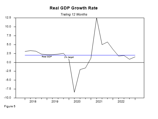
But everything else does not need to remain the same. So far, we have not discussed the demand for bank credit. If one is willing to use the real GDP growth rate as a proxy, then the real GDP outlook is critical to this analysis. If there is no recession and the economy continues to expand, we expect the demand for credit to expand and interest rates to rise. But is that a sure thing? Not by a long shot. Just look at Figure 4 where the peak in the bank credit multiplier leads the peak in the bond yields. But is this related to the pace of economic growth? Notice in Figures 4 and 5 that the trough in bond yields coincided with the COVID shutdown and the decline in economic activity documented in Figure 5. As the economy recovered, we contend that the demand for credit rose and so did bond yields, although the pace of economic activity declined the economy continued to expand. However, once the pace of economic activity began to hover at or below the 2% real GDP growth rate, the demand for credit and concerns about a recession began to emerge, the bond yields and bank credit creation peaked around the same time.
Our outlook is that as the inflation rate approaches the 2% target range, we expect the T-bill yields to stabilize. At the long end of the spectrum, the interest rates are driven by more than inflation, the pace of economic activity matters a great deal. Since the economy has shown signs of weakening, the long-term bond yields have declined. The combination of slower growth and declining inflation rate have contributed to the decline in bond yields. Since the beginning of the year these two variables have moved in tandem. But we do not expect that to continue on for long. The trend in the inflation rate points to a slowdown or less aggressive Fed stance. The deceleration in M2 supports this view. Then, at some point, we expect the economy to return to its normal trendline and with some luck even surpass the “new normal.” This expected divergence between the growth rate and inflation rate should result in a higher bond yield and a normalized yield curve.

IMPORTANT DISCLOSURES
The information in this report was prepared by Timber Point Capital Management, LLC. Opinions represent TPCM’s and IPI’s opinion as of the date of this report and are for general information purposes only and are not intended to predict or guarantee the future performance of any individual security, market sector or the markets generally. IPI does not undertake to advise you of any change in its opinions or the information contained in this report. The information contained herein constitutes general information and is not directed to, designed for, or individually tailored to, any particular investor or potential investor.
This report is not intended to be a client-specific suitability analysis or recommendation, an offer to participate in any investment, or a recommendation to buy, hold or sell securities. Do not use this report as the sole basis for investment decisions. Do not select an asset class or investment product based on performance alone. Consider all relevant information, including your existing portfolio, investment objectives, risk tolerance, liquidity needs and investment time horizon.
This communication is provided for informational purposes only and is not an offer, recommendation, or solicitation to buy or sell any security or other investment. This communication does not constitute, nor should it be regarded as, investment research or a research report, a securities or investment recommendation, nor does it provide information reasonably sufficient upon which to base an investment decision. Additional analysis of your or your client’s specific parameters would be required to make an investment decision. This communication is not based on the investment objectives, strategies, goals, financial circumstances, needs or risk tolerance of any client or portfolio and is not presented as suitable to any other particular client or portfolio. Securities and investment advice offered through Investment Planners, Inc. (Member FINRA/SIPC) and IPI Wealth Management, Inc., 226 W. Eldorado Street, Decatur, IL 62522. 217-425-6340.
Recent Comments